Fundamental Investigations of Gas Chromatography

Theory

Gas chromatography is a broad term that includes the very popular gas-liquid chromatography (partition) and gas-solid chromatography (adsorption). It ranks as one of the most important and versatile instrumental techniques since its invention in 1952. Prior to that date, separation of close boiling volatile liquids was impossible by conventional distillation, however, then new technique by Martin and Synge then by Martin and James allowed for simple separation of species such as benzene and cyclohexane (bp 80.1 and 80.8℃).

Separation occurs by passing the sample vapour dissolved in a carrier gas or mobile phase past a stationary support consisting of a solid (firebrick (Chromosorb-P or W) or diatomaceous earth) coated with a thin liquid layer. The theory of layer thickness will be featured in a brilliant lecture on the subject and will not be entertained here. As the sample vapours pass, the sample equilibrates or partitions into this liquid layer with each equilibration zone being called a ‘theoretical plate’. One of our goals in this experiment is to find the plate height at optimum flow using this instrument. Obviously, the equilibration of different sample will occur in different size zones, thus each will have their own optimum flow rate depending on the identity of the liquid layer.

The mechanism of separation is two fold. First is species bp and their desire to remain dissolved in a liquid vs dissolved in a gaseous layer. Smaller very volatile species will tremendously favor the gas layer and thus will depart the column more rapidly than a larger and lower volatility species. The secondary mechanism is via polarity. As the liquid layer is made (purchased) in a more polar derivative, a more polar sample will be retained longer in the liquid than a similar size nonpolar species. These two methods will be used to separate the species in a multicomponent mixture. The six most common liquid layers are listed in Table 1. This is not an all inclusive list!

Table 1 Top six commercial liquid layers for gas chromatography.

Column liquid	Tmax, ℃	Commercial examples
Dimethylsiloxane	350	OV-101, SP-2100, SE-30
50 % phenyl methyl silicone	375	OV-17, SP-2250
Polyethylene glycol	225	Carbowax 20M
Diethyleneglycol succinate (DEGS)	200
3-Cyanopropyl silicone	275	Silar 10-CP, SP-2340
Trifluoropropylmethyl silicone	275	OV-210, SP-2401

As you probably recall from Quantitative Analysis, there are several other important parts to a simple GC. Sample must be injected onto the column via an injection port that is usually maintained approximately 50 ℃ higher in temperature than the column to allow for flash vaporization. The vapour is scooped by carrier gas and carried into and through the column upon whose exit appears the detector, also maintained at 50 ℃ over the column temperature to prevent condensation of the sample onto the detector. The textbook has some excellent discussions on the detectors for GC. The Bloomsburg campus has five (depending on the day) research grade GC units:

1. an Agilent 8890 GC-MS

2. an Agilent 8860 with autosampler and FID

3. a Hewlett Packard 6890 with autosampler and FID

4. a ThermoScientific Focus with FID, and

5. a ThermoScientific Trace GC with thermal conductivity (TCD)/electron capture (ECD) and flame ionization (FID) detection.

All, of course subject to change — so look at the box on the bench!

Experimental

Apparatus

• Agilent 8890 GC-MS

• syringe, 10 μL

• tank of helium with regulator

Chemicals

• Chloroform (reagent grade or better)

• Carbon tetrachloride (reagent grade or better)

Determination of the Optimum Flow Rate in Gas Chromatography

Theory

Good separation by GC depends on proper control of many variables including judicious selection of a column substrate and on the overall efficiency of the entire GC system. Column efficiency is concerned with the broadening of an initially compact band (or slug) of solutes as it passes through the column. Broadening is the result of the column design and of the operating conditions. Efficiency is described quantitatively as the height equivalent to a theoretical plate (HETP or \(H\)), where a theoretical plate is defined as the length of column necessary for the attainment of solute equilibrium between the mobile and stationary phases. As HETP will depend on solvent, solute, temperature, flow rate, and sample size, these variables must be specified in order to compare efficiencies. HETP is used to compare columns or set standards for packing techniques. It is theoretical, however, thus can not be used as an absolute measure of a columns separating ability.

The value of HETP depends on the number of theoretical plates found on a column (\(N\)) and the overall length of the column (\(L\)) and is calculated by:

(9)\[H = \frac{L}{N}\]

The plate number, \(N\), can be determined from the chromatographic output:

(10)\[N = \left( \frac{4 t_r}{w_b} \right)^2\]

where \(t_r\) is the retention time and \(w_b\) is the peak width measured at the base. Another method of calculating N uses the peak width value at half-height:

(11)\[N = 5.54 \left( \frac{t_r}{w_{1/2}} \right)^2\]

These latter equations are identical based on statistical probability of a gaussian peak.

The number of theoretical plates is affected by three variables: sample injection, column characteristics, and detector volume. The sample should be injected as rapidly as possible and be flash vaporized. This will generate a small coherent band of sample with no tail. If the sample size is too large, the vaporization for part of the sample will lag behind the early material; resulting in a poor initial slug of material and often overloading of the column. As well spoken bearded analytical chemist likes to say — “the peak can’t get any narrower than what you injected”.

Columns can affect a separation before they are taken out of the box. A thick liquid layer will always lead to wider peaks than a thinner liquid layer of the same material. Particle size of the support will affect the separation as will the orderliness of the packing. Once a column is purchased, the flow rate is a very important variable in determining how well a separation will work. Three types of diffusion are important for a GC separation (and 5 for a LC thus we will use GC). The first type is longitudinal or concentration diffusion. All species flow from a larger to lower concentration thus as the band of sample travels down the column, it is diffusing both with and against the carrier gas flow causing peaks to be broader. The longer the retention time, the more broadening will occur, thus this type of diffusion can be decreased with a higher flow rate or temperature. The second type of broadening can now appear, mass transfer between the two phases is not a constant thus the partitioning will take more of the column and efficiency will drop. The third type of diffusion is eddy diffusion, the randomness of paths that a solute can take while traveling down the column, each with a different length thus each with a different retention time. This effect is smaller with smaller particles and with more regular packing of those particles.

These three effects are summarized by the van Deemter equation which can be simplified[1] to:

(12)\[H = A + \frac{B}{μ} + Cμ\]

where \(μ\) is the flow rate, \(A\) is the eddy diffusion term, \(\frac{B}{μ}\) is the longitudinal diffusion term, and \(Cμ\) is the mass transfer rate term. The van Deemter equation is plotted (\(H\) vs. \(μ\), Fig. 13) to yield a flow rate with a minimum value of \(H\) thus highest column efficiency. Values for the various terms can also be obtained from the plot. By extrapolating the non-attainment of partition equilibrium line to \(μ=0\), where the value of \(H\) equals the \(A\) term. The slope of the line used to extrapolate \(μ=0\) is the value of \(C\). To find the last term, \(B\), the equation must be differentiated with respect to \(μ\) and set equal to zero

(13)\[\frac{\partial{H}}{\partial{μ}} = -\frac{B}{μ^2} + C\]

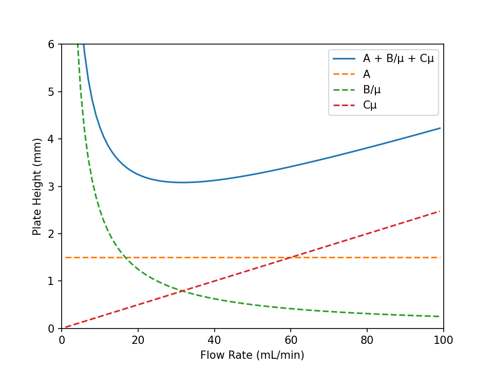
Fig. 13 A plot of the van Deemter equation and each individual term. Values of \(A = 1.25\,\text{mm}\), \(B = 25\,\text{mm}\), and \(C = 0.025\,\text{mm}\) were used. Adapted from Wikipedia, user Pronchik.

At \(μ_{\text{OPT}}\), each side of the expression must equal zero:

(14)\[\frac{\partial{H}}{\partial{μ}} = 0 \qquad\text{and}\qquad -\frac{B}{μ_{\text{OPT}}^2} + C = 0\]

therefore,

(15)\[B = Cμ_{\text{OPT}}^2\]

Procedure

1. Make sure you understand the operation of the GC instrument. Set up the GC for operation. Your instructor will indicate the appropriate literature to review prior to the experiment.

2. Connect the soap bubble flow meter to the exit gas port from the TCD detector. Determine the flow rate using the on board stop watch and converter.

   Note

   The Agilent 8890 GC-MS does not have a TCD detector. Instrument needs may change which GC we’re using. Modern instruments have an EPC that can adjust the flow rate as necessary as well as report this value to you.

3. Obtain chromatograms of pure chloroform using 1.0 μL injections at at least 6 different flow rates.

   Attention

   After changing the flow rate, wait several minutes before injecting the samples and officially measuring the flow rate. This ensures the system equilibration is completed.

   Measure flow rate both before injection and after the sample has been eluted.

Treatment of Data

1. Convert flow rates to milliliters per minute (if needed).

2. From the chromatogram and the column length, calculate the value of \(H\) at each flow rate then construct a van Deemter plot as in Fig. 13. Set the instrument to the optimum flow for Quantitative Analysis of Mixtures by Gas Chromatography. Calculate values for \(A\), \(B\), and \(C\) terms.

Questions

1. A hydrocarbon gave a GC peak for which \(w_{1/2}\) = 0.60 s and \(t_r\) = 0.92 min. Calculate the plate number and \(H\) given a column length of 10 meters.

2. Show what effect an increase in gaseous diffusion coefficient of a solute in the carrier gas would have on the longitudinal diffusion curve in Fig. 13.

3. A mixture of four hydrocarbons is to be separated. A van Deemter plot is obtained for one of the hydrocarbons and the flow rate is set at the minimum value in the plot. Does this flow rate also give the minimum value for \(H\) for the other three hydrocarbons? Explain.

4. Would \(μ_{\text{OPT}}\) increase or decrease if the column temperature is increased? Explain.

Quantitative Analysis of Mixtures by Gas Chromatography

Theory

Gas chromatography is widely used for quantitative analysis of gases and volatile liquids. The area under the curve for a species is proportional to the concentration of the species. Obtaining a calibration curve of concentration vs peak height or peak area leads directly to the unknown concentration. Similarly, use of an internal standard and plotting ratio of species to standard concentration can help remove instrumental and environmental errors. One major limitation is the volume of sample actually injected into the chromatograph.

When dealing with a binary mixture, this limitation can be circumvented by constructing a calibration curve in which the area or peak height ratio for the two components is plotted against a function of the sample concentration. The ratio has the advantage that it should be independent of the sample volume. If \(R\) represents the volume fraction of component #2 in the binary mixture, then

(16)\[R = \frac{S_2A_2}{S_1A_1 + S_2A_2}\]

which rearranges to:

(17)\[\frac{1}{R} = \frac{S_1A_1}{S_2A_2} + 1\]

Therefore, if the area ratio (\(\frac{A_1}{A_2}\)) is plotted against \(\frac{1}{R}\), a straight line of slope \(\frac{S_1}{S_2}\) should result which passes through the point \(\frac{A_1}{A_2} = 0\), \(\frac{1}{R} = 1\). (For example, a prepared known sample that contains 40% of component #2 and 60% of component #1 shows that \(\frac{1}{R} = 2.5\). By taking known volume rations and measuring their area ratios, a calibration curve can be constructed). Accordingly, when the area ratio of an unknown mixture is is measured, the corresponding value of \(\frac{1}{R}\) can be read from the calibration curve and the composition can be calculated.

Procedure

Adjust the flow rate of the chromatograph to the optimum value for chloroform found above. Prepare a series of standard solutions of chloroform and carbon tetrachloride that contain 30, 40, 50, 60, and 70 % chloroform by volume. Obtain chromatograms of each of the mixtures and of an unknown sample obtained from the instructor.

Treatment of Data

Construct a ratio calibration curve from both the peak heights and areas of the standards. Use theory and your noodle to determine which species is which! Use this curve to determine the makeup of the unknown.

Questions

1. Explain the order of elution of chloroform and carbon tetrachloride from the chromatograph.

2. Do you expect methylene chloride (1,2-dichloromethane) to elute faster or slower than the chloroform? Why?

3. What would happen to chromatographic output if temperature were decreased between successive runs?

References

• Dal Noare, S. And Juvet, R.S., Jr.,Gas Liquid Chromatography, Interscience:New York, 1959.

• Keulemans, A.I.M.., Gas Chromatography, Second Edition, Reingold: New York, 1959.

• Purnell, H., Gas Chromatography, Wiley: New York, 1962.

• Any undergraduate instrumental textbook.

[1]

Fear not — we will derive the full van Deemter equation in lecture (if that has not already occurred)!